Modelwerk: Beyond Transformers
The last and two most interesting models in the modelwerk series turned out to be ones that came after the transformer. Not because they're better, but because they seek to answer the question 'what comes next?' in completely opposite ways. In this post we take a look at Mamba and Continuous Thought Machines (CTM).
Mamba says: simplify the mechanism. Replace the transformer's attention with a recurrence. Give the network three learnable knobs and let the data-dependence do the work. Perhaps we don't need to compare every token to every other token all the time. Perhaps a running state, updated selectively, is enough most of the time. The Continuous Thought Machine says: enrich the computation. Give every neuron its own internal temporal processor, let the network take multiple steps, and let it use temporal correlations between the neurons. Perhaps the network should not be forced to answer after just one inference pass. Perhaps some problems benefit from having internal time as part of the representation. Building them both from scratch, up from the same primitives and building block used for the first four provided intuition in a way that reading the papers doesn't.
Series recap
The previous post covered four networks as a series of lessons: perceptron (1958), multi-layer network with back-propagation (1986), LeNet-5 with convolutions (1998), transformers (2017). That progression traces a path through fixed computation → learned computation → spatial structure → learned attention. The earlier lessons had a neat pattern to them. Each architecture solved a problem the previous one could not solve. Perceptrons gave you a decision boundary. Backprop let the network learn hidden features. Convolutions made spatial structure a first-class construct. Transformers let each position inspect everything else and decide what to pay attention to. Each new model also increased the amount of compute. And everything after the transformer has to deal with two problems attention created: quadratic cost in sequence length, and fixed computation per input regardless of difficulty.
Mamba and the CTM each take one of those problems as their starting point. And so the next step was never likely to be more attention. It was going to be some new concept and some new way of spending compute.
Mamba: what if we didn't pay so much attention?
Attention is one of the most elaborate mechanisms in modern neural networking. Learned queries, keys, values, multi-head projections, causal masking, positional encoding: it's a lot of machinery. The transformer’s great move was to let every token look at every other token, and the cost of that move is by now well understood: self-attention scales quadratically with sequence length, which is fine until it isn’t. Mamba's argument is essentially: what if we replaced all of that with a recurrence that maintains a compressed running state, updated at each position in linear time. The new concepts it brings in are:
State space. Instead of attending to all positions (quadratic), maintain a hidden state h that summarizes the sequence so far. Each position updates h and reads from it. The cost is O(N) instead of O(N²).
Input-dependent selection. Classical state space models use fixed parameters, and process every token the same way, which limits them to fixed-spacing patterns, equivalent to convolutions. Mamba computes its parameters, Updates, Outputs, and Delta from the current input. Updates control what gets written into state, Outputs controls what gets read out, and Delta controls how much to write. This lets the model decide per token what to remember.
Delta as a gate. Delta is technically the discretization step size, but a way to think about it, is as a volume knob. High Delta means this is important, remember it. Low Delta means this is noise, skip it.
Discretization. This means the continuous-time math gets converted to discrete step-by-step updates via an Euler approximation. A detail that matters for the implementation but not for the intuition.
Mamba's state space model matters, but arguably the real novelty is selection. Earlier structured state space models had fixed dynamics and were time-invariant, which is a way of saying they were good at regular patterns and less good at information-dense symbolic sequences, like text. Mamba lets the state update depend on the token being processed, so the model can decide, token by token, what deserves to be written into state and what can be ignored. In short attention says, 'look everywhere, then weigh it’, whereas Mamba says, 'have a memory, then decide whether this token changes it'.
In the lesson, the task we used to test the network, 'selective copying', is taken directly from the Mamba paper. Data tokens appear at random positions in a sequence of blanks. After a marker, the model must reproduce the data tokens in order. The randomized spacing is the whole point a fixed-parameter model can solve regular copying by learning to matches the fixed offsets, but random spacing kills any chance of using fixed-pattern shortcuts. The model has to inspect each token to decide whether to remember it.
The useful teaching moment for me at least was that Mamba became understandable when we stopped treating it as an anti-transformer and started treating it as a very specific answer to one problem: how do you keep long-range sequence modeling without paying the full O(N²) cost of attention? The mechanism is actually fairly restrained. There’s the recurrence (a sequence of steps), some learned projections, and the discretization step in Delta.
That also affected the implementation. The forward pass is not simple exactly, but it is narratable. A compressed state moves left to right through the sequence. Delta decides how open the write path is and Updates and Outputs decide what gets written and how it gets read back out. Once you have that task in front of you in code, the idea of an input-dependent write gate clicks: the machine has to learn to 'notice' the data tokens and not the blanks.
The delta heatmap
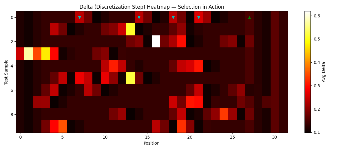
When the model was behaving properly, the diagnostic plots became legible: Delta spikes around where the meaningful tokens are, idles on blanks, and the state carries the payload forward. The delta heatmap is where you can see the selection mechanism working:
Data token positions light up (Delta values of 0.18–0.62) while blanks stay at baseline (0.11–0.13). Sample 2 is particularly good: Delta hits 0.62 at position 16, the highest spike in any sample. The tokens at positions 13, 16, and 18 are close together, and the model learned to gate more aggressively when data arrives in quick succession — it needs to write harder because the state is already occupied with recent content. The model learned, from gradient signal alone, to open its gate at data tokens and keep it shut at blanks. No one told it which tokens mattered. It figured out the distinction from the copying loss.
Training Mamba
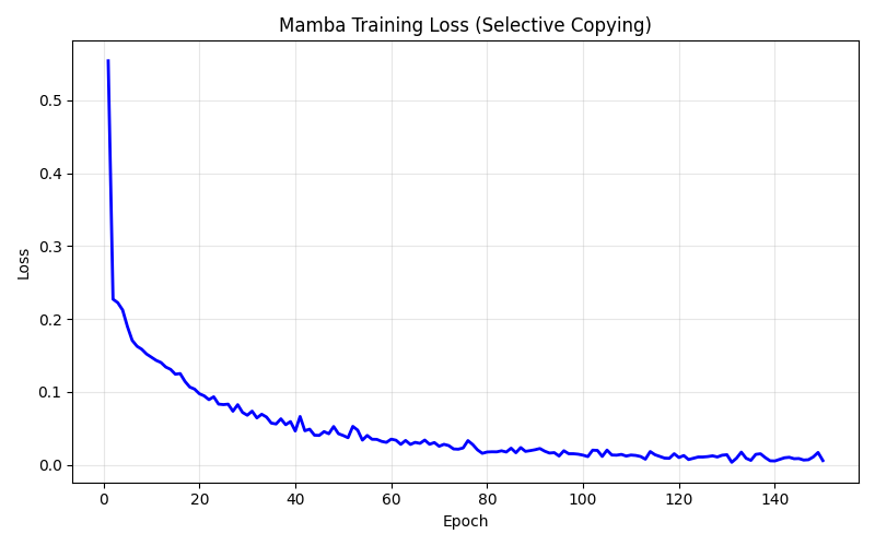
The training curve is smooth, no mysterious basin-hopping, instability, or loss spikes, just a steady monotonic descent from 0.55 to 0.006 over 150 epochs. The rapid initial drop (0.55 → 0.08 in 25 epochs) is the model learning to predict blanks at most positions. The slower descent from there is the model refining its selective copying: learning when to spike delta, what to write into state, how to read it back in order. The lesson's 5,936-parameter model reached 89% token accuracy and 64% full-sequence accuracy. My understanding is the misses are almost entirely down to token re-ordering, where the model captures the right tokens but occasionally confuses their ordering. The 8-dimensional hidden state is encoding both identity and position for 4 tokens; when two data tokens have similar spacing relative to the copy marker, the position encoding can blur.
Why Mamba matters
Mamba is interesting because it actively removes a complication, attention. Three learnable knobs, a recurrence, and the data-dependence does the work. Efficiency here is not a detail. Linear-time sequence modeling changes what lengths and workloads are tractable, and that is why these models keep showing up in the conversation. The research results bear this out. Mamba-3 was recently published at ICLR 2026, and the numbers are real: linear scaling in sequence length, constant memory at inference, and Mamba 3B matching transformer accuracy at roughly double the parameter count. The production story is evolving too. Jamba (transformer + Mamba + Mixture of Experts) is getting traction, and one emerging consensus seems to be that the future isn't 'Mamba replaces transformers' but something more pragmatic: Mamba layers handle the long-range stuff, attention layers handle the precise recall. Hybrids rather than replacements.
Continuous Thought Machines: what if we gave the network time to think?
The CTM comes at the post-transformer problem from another direction. Instead of making sequence processing cheaper, it makes computation adaptive. The network runs for T internal ‘thought steps’, or ticks, refining its answer at each tick, and learns on its own what to output. A transformer has depth, but it is fixed depth, where a hard example and an easy example both get the same number of layers. Chain-of-thought prompting, thinking step by step, and search methods try to bolt extra reasoning on from outside. CTM says that perhaps iterative computation should be native to the network, not external. The idea is let the model have its own internal thinking steps, and let the representation live not only in activations but in how neurons synchronize with each other over time. The new concepts are:
Internal time. The network loops, or ticks, T times over the same input. Each tick can change what the network attends to and refine its answer. Easy inputs get fast answers; hard inputs get more thinking. The model refines its state and predictions over time rather than producing one answer in one pass.
Neuron-level models. Instead of a neuron holding just an activation triggered by a nonlinear function, every neuron has its own private multi-layer network that processes a rolling history of its past activations. This gives each neuron the capacity to develop its own temporal behavior.
Neural synchronization. The representation isn't neuron activations but their temporal correlations. Two neurons with the same activation at tick t carry different information if one has been oscillating and the other has been steady. A sync vector captures that distinction. With N neurons in a sync group, you get N² pair correlations encoding patterns across the full tick history.
Certainty-based loss. The network predicts at every tick, but the loss function for training only uses two: the one with lowest loss and the one with highest certainty. Adaptive compute emerges without an explicit halting mechanism.
In an ordinary network, a neuron is an object where a weighted sum gets transformed and passed along. In CTM, the neuron starts to have a disposition, and can respond based on what it has been through over the last few ticks, not just what arrived this instant.
The synchronization mechanism makes that really interesting. Two neurons with the same current activation can mean different things if one got there through steady buildup and the other by oscillation. Activations collapse that history, the neurons will just fire based on the inputs. Synchronization preserves what they did at a particular time. The model gets extra representational room from the time relationships between neurons.
The parity task from the paper is a good test for this architecture. Each input is a sequence of +1 and -1 values; the target is the running parity. The answer depends on the entire input, and difficulty scales with length, exactly the kind of problem where iterative refinement should pay off.
The optimizer as design constraint
What made CTM particularly valuable in modelwerk was not that it dropped into place cleanly. It definitely did not. The most educational part of building the CTM was discovering that the AdamW optimiser used in the paper isn't optional—it's load-bearing.
The first cut used stochastic gradient descent (SGD), which we have from previous lessons, and is a go to optimiser. SGD more or less failed consistently, plateauing in the same rough region, getting to a loss ~0.6 and staying clamped to there. I tried a few things like dropping the learning rate and increased the epochs, but it wasn't a tuning problem. In retrospect I should have known that consistent failure is telling you something structural rather than incidental. In this case it meant CTM's different parameter groups genuinely live at different scales: decay rates are scalars that control how far back synchronization remembers, the NLM weights are 32 tiny private networks, the synapse is a shared MLP, and the attention projections are standard dense layers. The single learning rate provided by SGD which treats all parameters can't serve all of them. The 0.6 plateau was SGD finding the best compromise learning rate and then getting stuck because that compromise is bad for every group.
It made sense to try AdamW, which is what paper uses. The next attempt using AdamW and clipping the magnitudes, was better getting to up to around 55% accuracy, directionally correct, but still not good. Once we let it off the hook, it hit 95%. Gradient clipping actually hurt, because AdamW's per-parameter scaling was already handling the magnitude problem, and clipping was interfering with it.
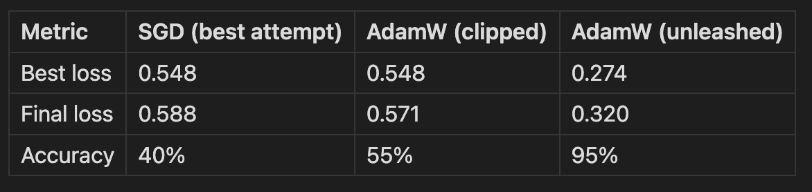
That jump, from 40% to 95% is the difference between 'not working' and 'working.' That was probably the best learning moment in the whole project: not because it was surprising that one optimizer beat another, but because the way SGD failed suggested why: the parameter groups are doing genuinely different jobs and living on different scales. AdamW is able to optimise individual parameter groups differently which gave CTM the flexibility it needed. The paper kind of buries it: "AdamW, lr=1e-4" in an appendix table, but the architecture is borderline hostile to approaches like SGD. This was the first network in the series I had to genuinely tune and debug before it became usable as a lesson, and that itself felt instructive. All the previous models were about developing insight and ensuring the material and code could teach, but the CTM required operational troubleshooting to get it working.
The certainty heatmap
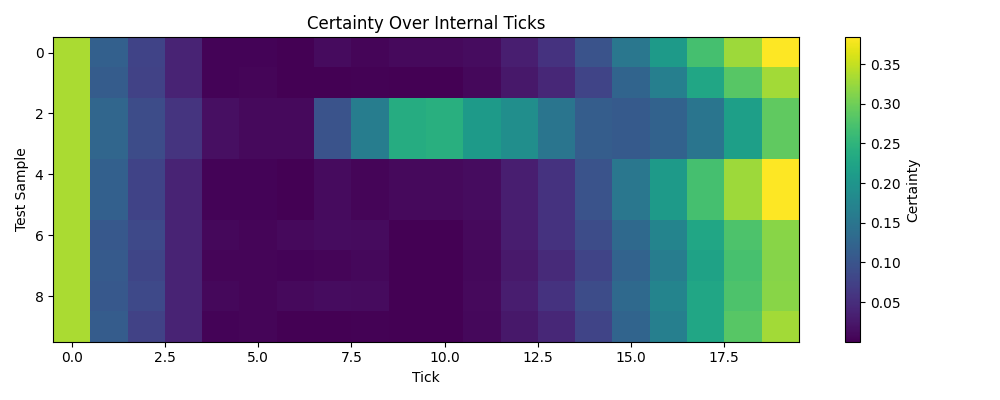
The certainty heatmap shows how confidence evolves across the 20 internal ticks for each test sample. Tick 0 is bright; the initial state gives a non-trivial starting prediction before any thinking has happened (this is learned: the model discovers that its initial state can encode a useful prior). The middle ticks go dark as certainty collapses. The network is efining its state over internal ticks, exploring the input through attention mechanics, and updating its running estimates. Then certainty recovers in later ticks as the model converges on an answer. Different samples have different profiles. Some develop certainty early; others stay dark until the final ticks. The network learned when to commit.
Synchronization: a deeper innovation?
The idea that seems to get the most attention in discussions of the CTM is ‘each neuron has its own brain’, however synchronization is doing a lot of the heavy lifting. Using temporal correlations as the representation rather than the activations themselves means the model has access to a richer space. The dimensionality expansion comes from time rather than from width. With N neurons in a sync group, you get N² pair correlations, and those correlations encode patterns across the full tick history. The network's representation lives in the temporal relationships between neurons over time. This is how just 5,794 parameters can do what they do: the tick loop reuses the synapse and attention weights 20 times, and the sync mechanism extracts N² signals from N neurons without needing additional parameters.
Training dynamics
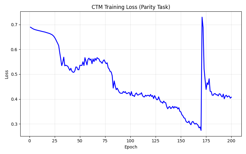
The CTM's training curve is revealing when you put it next to Mamba's. The CTM’s loss dropped in stages, breaking out of the initial plateau around epoch 30, a longer descent through the 0.4s, reaching a minimum around epoch 170. Then a sharp spike as the model hits an unstable gradient configuration, and a partial recovery. It’s non-monotonic, with clear phase transitions. By comparison, Mamba's recurrence is a linear update where gradients flow through element-wise, and are stable by construction. The CTM has five interacting mechanisms all coupled through the tick loop, with six gradient chains running simultaneously through back-propagation. Most ticks get zero direct loss gradient. Instead they learn entirely through the state chains: if a middle tick changes its state slightly, that changes the next tick's input, which eventually changes the output at a supervised tick. The backwards pass is where you can see the engineering detail and complexity: it’s easily the most involved code in the series.
There was also a genuine bug in the backward pass that Codex found via a review. The gradients for the embedding projection and its key-value weights were initialized to zeros and never accumulated : the chain from cross-attention stopped at the projection matrices instead of continuing back through layer norm to the embeddings. Three parameter groups training from random initialization the entire time. Fixing it was straightforward. But on rerun, confidence went up and performance collapsed. Turns out, the model was overfitting because the training data set was so small. The bug had been acting as a regularizer, freezing those weights limited the model's capacity just enough to match the tiny dataset. The correct gradient chain produces a worse model because the data can't support it. More complete gradients aren't always better when data is scarce. The fix was backed out with a note, because the lesson runtimes could push into 30 minutes.
Why CTM matters
The CTM is a bet that networks should learn their own thinking process. Right now, deliberation in AI is more or less hand-engineered: chain-of-thought prompting, tree search, step by step, scratchpads. The parallel to computer vision in lesson 3 is hard to ignore. Before ConvNets, people hand-designed spatial features, such as edge detectors, SIFT, or Haar cascades. Convolutions let the network learn its own spatial structure, and that paid off because spatial locality is a true prior about visual data. The CTM makes the same move for computation itself: let the network learn certainty peaks at different ticks for different samples longer, and what to select. The parity result: 95% accuracy from 5,794 parameters, with adaptive compute emerging from the loss function, is a signal that temporal synchronization might in turn be a true prior about deliberation: the model genuinely learned to think longer on harder problems. It's early, and the engineering is demanding. But the direction is worth watching.
Where complexity goes
There's a design archetype that shows up in some architectures: the complexity lives in the interaction between mechanism and data, not always in the mechanism itself. Attention is like this; the interaction between learned queries and learned keys produces rich behavior. Mamba's selection follows the same pattern, a recurrence becomes powerful because it’s data-dependent: three tunables, and the data does the rest. The CTM spends computation differently. Scalar decay rates, per-neuron networks, a shared synapse, dense attention projections — each with its own magnitude and learning dynamics. The architecture asks more of the optimizer and the training signal than anything else in the series. Mamba asks: how cheaply can we process a sequence while still being selective? The CTM asks: what happens when a network gets to decide how much to think? The first question has clearer production implications today; the second might matter more in the longer run.
Closing
The modelwerk series progression now reads: fixed computation → learned computation → spatial structure → learned attention → efficient selection → internal time. From a single perceptron neuron to models that choose what to remember and when to stop thinking. Each of these six lessons has a ‘what can this do that the previous thing couldn't’ moment. For the perceptron it was limited to linear classification. For the multi-layer network with back-propagation, non-linear XOR. For the LeNet-5 ConvNet with gradients, spatial features. For the transformer, arbitrary dependencies. For Mamba, linear-time selection. For the CTM, time. Like we said at the beginning, building them from scratch using only standard Python, provided real insight. You get to see in the code what each architecture is trying to do, what new ideas it introduces, the structure and where the extra capability comes from.
Six papers, spanning nearly seventy years. Every operation is Python code traceable from the model down to scalar multiply. The models are slow, the data is tiny, the code is naive. But none of that matters: what matters is that you can see the machinery.